Do Machine Learning Models Memorize or Generalize?

By Adam Pearce, Asma Ghandeharioun, Nada Hussein, Nithum Thain, Martin Wattenberg and Lucas Dixon

August 2023

In 2021, researchers made a striking discovery while training a series of tiny models on toy tasks . They found a set of models that suddenly flipped from memorizing their training data to correctly generalizing on unseen inputs after training for much longer. This phenomenon – where generalization seems to happen abruptly and long after fitting the training data – is called grokking and has sparked a flurry of interest .

Do more complex models also suddenly generalize after they’re trained longer? Large language models can certainly seem like they have a rich understanding of the world, but they might just be regurgitating memorized bits of the enormous amount of text they’ve been trained on . How can we tell if they’re generalizing or memorizing?

In this article we’ll examine the training dynamics of a tiny model and reverse engineer the solution it finds – and in the process provide an illustration of the exciting emerging field of mechanistic interpretability . While it isn’t yet clear how to apply these techniques to today’s largest models, starting small makes it easier to develop intuitions as we progress towards answering these critical questions about large language models.

Grokking Modular Addition

Modular addition is essentially the fruit fly of grokking. The above line chart comes from a model trained to predict $a + b \bmod 67$ . We start by randomly dividing all the $a, b$ pairs into test and training datasets. Over thousands of training steps, the training data is used to adjust the model into outputting correct answers, while the test data is only used to check if the model has learned a general solution.

The model’s architecture is similarly simple: $\text{ReLU}\left(\mathbf{a}_{\text{one-hot}} \mathbf{W}_{\text{input}} + \mathbf{b}_{\text{one-hot}} \mathbf{W}_{\text{input}}\right) \mathbf{W}_{\text{output}}$ — a one-layer MLP with 24 neurons. All the weights of the model are shown in the heatmap below; you can see how they change during training by mousing over the line chart above.

The model makes a prediction by selecting the two columns of $\mathbf{W}_{\text{input}}$ corresponding to inputs $a$ and $b$ then adding them together to create a vector of 24 separate numbers. Next it sets all the negative numbers in the vector to 0 and finally outputs the column of $\mathbf{W}_{\text{output}}$ that’s closest to the updated vector.

The weights of the model are initially quite noisy but start to exhibit periodic patterns as accuracy on the test data increases and the model switches to generalizing. By the end of training, each neuron — each row of the heatmap — cycles through high and low values several times as the input number increases from 0 to 66.

This is easier to see if we group the neurons by how often they cycle at the end of training and chart each of them as a separate line:

The periodic patterns suggest the model is learning some sort of mathematical structure; the fact that it happens when the model starts to solve the test examples hints that it’s related to the model generalizing. But why does the model move away from the memorizing solution? And what is the generalizing solution?

Generalizing With 1s and 0s

Figuring out both of these questions simultaneously is hard. Let’s make an even simpler task, one where we know what the generalizing solution should look like and try to understand why the model eventually learns it.

We’ll take random sequences of thirty 1s and 0s and train our model to predict if there is an odd number of 1s in the first three digits. e.g. 000110010110001010111001001011 is 0 while 010110010110001010111001001011 is 1 — basically a slightly trickier XOR with some distraction noise. A generalizing model should only use the first three digits of the sequence; if the model is memorizing the training data, it will also use the subsequent distracting digits .

Our model is again a one-layer MLP, trained on a fixed batch of 1,200 sequences. At first only training accuracy increases — the model is memorizing the training data. As with modular arithmetic, test accuracy is essentially random and then sharply rises as the model learns a general solution.

While memorizing , the model looks dense and noisy with lots of high magnitude weights (shown as dark red and blue squares) spread across the chart below – the model is using all the inputs to make a prediction. As the model generalizes and gets perfect test accuracy, we see all the weights connected to the distracting digits gray out with very low values and the model focusing on the first three digits — mirroring the generalized structure we expected!

With this simplified example it’s easier to see why this happens: we’re pushing our model to do two things during training — output a high probability for the correct label (called minimizing loss ) and have weights with low magnitudes (known as weight decay ). Train loss actually slightly increases before the model generalizes as it exchanges loss related to outputting the correct label for having lower weights.

The sharp drop in test loss makes it appear like the model makes a sudden shift to generalization. But if we look at the weights of the model over training, most of them smoothly interpolate between the two solutions. The rapid generalization occurs when the last weights connected to the distracting digits are pruned by weight decay.

When Does Grokking Happen?

It’s important to note that grokking is a contingent phenomenon — it goes away if model size, weight decay, data size and other hyper parameters aren’t just right. With too little weight decay, the model can’t escape overfitting the training data. Adding more weight decay pushes the model to generalize after memorizing. Increasing weight decay even more causes test and train loss to fall together; the model goes straight to generalizing. And with too much weight decay the model will fail to learn anything.

Below, we’ve trained over a thousand models on the 1s and 0s task with different hyperparameters. Training is noisy so nine models have been trained for each set of hyperparameters.

We can induce memorization and generalization on this somewhat contrived 1s and 0s task — but why does it happen with modular addition? Let’s first understand a little more about how a one-layer MLP can solve modular addition by constructing a generalizing solution that’s interpretable.

Modular Addition With Five Neurons

Recall that our modular arithmetic problem $a + b \bmod 67$ is naturally periodic, with answers wrapping around if the sum ever passes 67. Mathematically, this can be mirrored by thinking of the sum as wrapping $a$ and $b$ around a circle. The weights of the generalizing model also had periodic patterns, indicating that the solution might use this property.

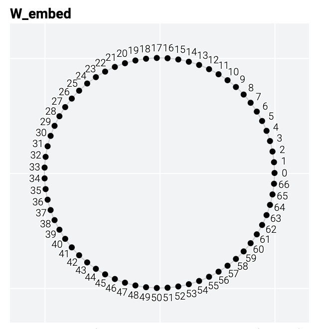
We can train a simpler model with a head start on the problem, constructing an embedding matrix that places $a$ and $b$ on a circle by computing $\cos$ and $\sin$ for each possible input number $i \in \{0, 1, \ldots, 66\}$ .

$\mathbf{W}_{\text{embed}} = \begin{pmatrix} \dots & \ldots \\ \cos(i\frac{2\pi}{67}) & \sin(i \frac{2\pi}{67}) \\ \dots & \dots \\ \end{pmatrix} \quad$

Then we train $\mathbf{W}_{\text{in-proj}}$ and $\mathbf{W}_{\text{out-proj}}$ in this one-layer MLP:

$\begin{aligned} \text{activations} & = \text{ReLU}\left(\mathbf{a}_{\text{one-hot}} \mathbf{W}_{\text{embed}} \mathbf{W}_{\text{in-proj}} + \mathbf{b}_{\text{one-hot}} \mathbf{W}_{\text{embed}} \mathbf{W}_{\text{in-proj}}\right) \\ \text{logits} & = \text{activations} \mathbf{W}_{\text{out-proj}} \mathbf{W}_{\text{embed}}^{\top} \end{aligned}$

With just five neurons the model finds a solution with perfect accuracy.

Eyeballing the trained parameters, all the neurons converge to roughly equal norms. If we directly plot their $\cos$ and $\sin$ components, they’re essentially evenly distributed around a circle:

Connect the adjacent neurons on the $\mathbf{W}_{\text{in-proj}}$ circle and an intriguing pattern emerges: $\mathbf{W}_{\text{out-proj}}$ is rotating around the circle twice as fast as $\mathbf{W}_{\text{in-proj}}$ .

The details of how this solution works aren’t essential — check out Appendix A to see how the doubled rotation allows the model to map inputs like $1 + 0 \bmod 67$ and $2 + 66 \bmod 67$ to the same place — but we have found a 20 parameter construction that solves modular addition. Can we find the same algorithm hidden in the 3,216 parameter model we started with? And why does the larger model switch to the generalizing solution after memorizing?

It’s Full of Stars

Here’s the $a + b \bmod 67$ model that we started with — it’s trained from scratch with no built-in periodicity.

Unlike the constructed solution, where $\mathbf{W}_{\text{embed}}$ rotates around the circle once, this model has many different frequencies.

Below, we’ve isolated the frequencies using the discrete Fourier transform (DFT). This factors out the learned periodic patterns across inputs, leaving us with the equivalent of $\mathbf{W}_{\text{in-proj}}$ and $\mathbf{W}_{\text{out-proj}}$ from the constructed solution. For each neuron, this gives a $\cos$ and $\sin$ value for every possible periodic frequency from 1 to 33. The wave charts we show above use this to group neurons into frequencies by finding their largest $\cos$ and $\sin$ value across all frequencies.

Just like in the 1s and 0s task, weight decay encourages this representation to become much sparser as the model generalizes .

Grouping neurons by their final trained frequencies, and plotting the $\cos$ and $\sin$ components of the DFT for each neuron, we see the same star shapes from the constructed solution appear.

This trained model is using the same algorithm as our constructed solution! Below, the contribution to the output generated by the neurons in each frequency are shown and we can see them calculating $\cos\frac{2\pi (a + b) freq}{67}$ .

Notice what happens to the group of neurons with a frequency of 7 when test loss improves after the short plateau at 45,000 steps — they start to snap into a star shape and their outputs more closely approximate a wave.

To lower loss without using higher weights (which would be punished by weight decay), the model uses several frequencies, taking advantage of constructive interference. There’s nothing magical about the frequencies 4, 5, 7 and 26 — click through other training runs below to see variations of this algorithm get learned.

Open Questions

While we now have a solid understanding of the mechanisms a one-layer MLP uses to solve modular addition and why they emerge during training, there are still many interesting open questions about memorization and generalization.

Which Model Constraints Work Best?

Directly training the model visualized above — $\text{ReLU} \left(a_{\text{one-hot}}\textbf{W}_{\text{input}} + b_{\text{one-hot}}\textbf{W}_{\text{input}} \right) \textbf{W}_{\text{output}}$ — does not actually result in generalization on modular arithmetic, even with the addition of weight decay. At least one of the matrices has to be factored:

$\textbf{W}_{\text{input}} = \mathbf{W}_{\text{embed}} \mathbf{W}_{\text{in-proj}}$

$\textbf{W}_{\text{output}} = \textbf{W}_{\text{out-proj}} \textbf{W}_{\text{embed}}^{\top}$

We observed that the generalizing solution is sparse after taking the discrete Fourier transformation, but the collapsed matrices have high norms. This suggests that direct weight decay on $\textbf{W}_\text{output}$ and $\textbf{W}_{\text{input}}$ doesn’t provide the right inductive bias for the task.

Broadly speaking, weight decay does steer a wide variety of models away from memorizing their training data . Other techniques that help avoid overfitting include dropout, smaller models and even numerically unstable optimization algorithms . These approaches interact in complex, non-linear ways, making it difficult to predict a priori which will ultimately induce generalization. Collapsing $\mathbf{W}_{\text{embed}} \mathbf{W}_{\text{in-proj}}$ instead of $\textbf{W}_{\text{out-proj}} \textbf{W}_{\text{embed}}^{\top}$ , for example, helps in some setups and hurts in others:

Why Is Memorization Easier Than Generalization?

One theory: there can be many more ways to memorize a training set than there are generalizing solutions. So statistically, memorization should be more likely to happen first, especially if we have no or little regularization. Regularization techniques, like weight decay, prioritize certain solutions over others, for example, preferring “sparse” solutions over “dense” ones.

Recent work suggests that generalization is associated with well-structured representations . However, it’s not a necessary condition; some MLP variations without symmetric inputs learn less “circular” representations when solving modular addition . We also observed that well-structured representations are not a sufficient condition for generalization. This small model (trained with no weight decay) starts generalizing, then switches to memorizing with periodic embeddings.

It’s even possible to find hyperparameters where models start generalizing, then switch to memorizing, then switch back to generalizing!

What About Larger Models?

Does grokking happen in larger models trained on real world tasks? Earlier observations reported the grokking phenomenon in algorithmic tasks in small transformers and MLPs . Grokking has subsequently been found in more complex tasks involving images, text, and tabular data within certain ranges of hyperparameters . It’s also possible that the largest models, which are able to do many types of tasks, may be grokking many things at different speeds during training .

There have also been promising results in predicting grokking before it happens. Though some require knowledge of the generalizing solution or the overall data domain , some rely solely on the analysis of the training loss and might also apply to larger models — hopefully we’ll be able to build tools and techniques that can tell us when a model is parroting memorized information and when it’s using richer models.

Understanding the solution to modular addition wasn’t trivial. Do we have any hope of understanding larger models? One route forward — like our digression into the 20 parameter model and the even simpler boolean parity problem — is to: 1) train simpler models with more inductive biases and fewer moving parts, 2) use them to explain inscrutable parts of how a larger model works, 3) repeat as needed. We believe this could be a fruitful approach to better understanding larger models, and complementary to efforts that aim to use larger models to explain smaller ones and other work to disentangle internal representations . Moreover, this kind of mechanistic approach to interpretability, in time, may help identify patterns that themselves ease or automate the uncovering of algorithms learned by neural networks.

Credits

Thanks to Ardavan Saeedi, Crystal Qian, Emily Reif, Fernanda Viégas, Kathy Meier-Hellstern, Mahima Pushkarna, Minsuk Chang, Neel Nanda and Ryan Mullins for their help with this piece.

Model training code // Visualization code

Appendix A: How the Circular Construction Works

We can almost calculate $a + b \bmod 67$ using two circular embeddings and a completely linear model.

It works! But we’re cheating a bit, do you see how unembed loops around the circle twice? We need to output a single prediction for ““ — not separate predictions for ““ and ““. Directly adding the two predictions for a number together won’t work since they’re on opposite sides of the circles and will cancel each other out.

Instead, let’s incorporate a $\text{ReLU}(x)$ to fix the repeated outputs.

We’ve essentially wrapped the circle around in on itself and the model outputs a single prediction for ““.

Formally, this is the constructed model:

With modulus $M$ and $N$ evenly spaced neurons/directions:

$\mathbf{W}_{\text{embed}} = \begin{pmatrix} \dots & \ldots \\ \cos(i\frac{2\pi}{M}) & \sin(i \frac{2\pi}{M}) \\ \dots & \dots \\ \end{pmatrix}, \quad \mathbf{W}_{\text{in-proj}}^T = \begin{pmatrix} \dots & \ldots \\ \cos(i\frac{2\pi}{N}) & \sin(i \frac{2\pi}{N}) \\ \dots & \dots \\ \end{pmatrix}, \quad \mathbf{W}_{\text{out-proj}} = \begin{pmatrix} \dots & \dots \\ \cos(2i\frac{2\pi}{N}) & \sin(2i\frac{2\pi}{N}) \\ \dots & \dots \\ \end{pmatrix}.$

Interestingly this circle has a few wrinkles: this construction doesn’t give an exact answer!

Neurons Modulus

Using $x^2$ instead of $\text{ReLU}(x)$ as the activation function, as suggested by gives a provably exact solution!

For simplicity, let $\omega:=\frac{2\pi}{M}$ (the angle between numbers in $\mathbf{W}_{\text{embed}}$ ) and $\theta := \frac{2\pi}{N}$ (the angle between neurons in $\mathbf{W}_{\text{in-proj}}^T$ ).

Let’s rewrite $\text{logits}^{a, b}$ as an $M$ -dimensional vector $\lVert \it{l} \rVert ^M$ where:

$l_{j} = \sum_{i=0}^{N-1} \biggl(\bigl[ \cos(a\omega-i\theta) + \cos(b\omega-i\theta) \bigl]^2\cos(j\omega-2i\theta)) \biggr)$

This follows from the $\text{logits}^{a,b}$ equation above by plugging in the definitions of $\textbf{W}_\text{in-proj}$ and $\textbf{W}_\text{out-proj}$ and applying the trigonometric identity that $\cos(x)\cos(y) + \sin(x)\sin(y) = \cos(x-y)$ .

We can then prove the following:

$\argmax_c \! \text{logits}^{a,b} = a + b \bmod M$

Applying the two trigonometric identities of $\cos(x) + \cos(y) = 2 \cos(\frac{x-y}{2}) \cos(\frac{x+y}{2})$ and $\cos^2(x)cos(y) = 1/4 \bigl[ 2\cos(y) + \cos(2x-y) + \cos (2x+y) \bigl]$ , we have:

$\begin{aligned} \text{logits}^{a, b} & = \sum_{i=0}^{N-1} \biggl(\bigl[ \cos(a\omega-i\theta) + \cos(b\omega-i\theta) \bigl]^2 \cos(c\omega-2i\theta) \biggl) \\ & = \sum_{i=0}^{N-1} \biggl(2 \bigl[ \cos(\frac{a-b}{2}\omega)\cos(\frac{a+b}{2}\omega-i\theta) \bigl] ^2 \cos(c\omega-2i\theta) \biggl) \\ & = \cos^2(\frac{a-b}{2}\omega) \sum_{i=0}^{N-1} \biggl(2\cos(c\omega - 2i\theta) + \cos((a+b-c)\omega) +\cos((a+b+c)\omega-4i\theta) \biggl) \end{aligned}$

Note that $\sum \cos(\gamma_{i})=0$ where $\gamma_{i}$ is equally spread around the circle. The first and the third sum terms wrap around the circle with $2\theta$ and $4\theta$ increments respectively. The sum of the first terms equals zero for $N \gt 2$ and the sum of the third terms equals zero for $N \gt 4$ . Therefore, we have:

$\text{logits}^{a,b} = \cos^2(\frac{a-b}{2}\omega) \cos((a+b-c)\omega)$

Since the first term is a positive constant w.r.t inputs, the equation is maximized when $\cos((a+b-c)\omega)$ is maximized, which is when $c = a + b \bmod M$ .

Essentially $\text{ReLU}(x)$ activations with weight decay (a very typical model setup) gives the model an inductive bias that’s close enough to the exact generalizing solution of $x^2$ activations with a sparse discrete Fourier transform to push in the direction of generalization but not so close that it won’t also learn to fit the training data with memorization.

Footnotes

In modular addition, we have two input numbers, $a$ and $b$ , and a modulus $m$ . We want to find the remainder of $a + b$ when divided by $m$ . This type of addition is often called clock-face addition, because when adding two times, we often report the result modulo 12 (i.e. 5 hours after 8 o’clock is 1 o’clock). Modular addition sounds simple and it is. We can easily train 1,000s of models and treat them like fruit flies in neuroscience: small enough such that it is feasible to extract their connectome synapse-by-synapse, yet providing new interesting insights about the system more broadly. We can get a good understanding of the small models we’ve trained by visualizing all their internals.

67 isn’t a magic number – we could pick many numbers to illustrate grokking, but 67 is not so small that the task is trivial and also not so large that the visualizations are overwhelming.

The model is trained with cross-entropy loss, AdamW and full batches. The section on regularization and training colab have additional details. If you’re not familiar with MLPs, playground.tensorflow.org is a great place to start. A quick notation explanation: The columns of $\mathbf{W}_{\text{input}}$ and $\mathbf{W}_{\text{ouput}}$ represent the numbers from 0 to 66. $\mathbf{a}_{\text{one-hot}}$ and $\mathbf{b}_{\text{one-hot}}$ are how we encode the model’s inputs; each pick a single column from $\mathbf{W}_{\text{input}}$ . $\text{ReLU}$ replaces negative numbers with 0s; it is a fancy) way of writing $\max(x, 0)$ .

With a small twist — we’re only outputting 1 or 0, so $\mathbf{W}_{\text{output}}$ can be a single column. In the modular addition task we needed a column for every output number. The last column of $\mathbf{W}_{\text{input}}$ is also fixed to 1 to provide a bias term.

Appendix D of “A Tale of Two Circuits: Grokking as Competition of Sparse and Dense Subnetworks” has an explanation of the 4 neuron solution generalizing solution here

So far we’ve been charting accuracy, the percentage of sequences where the correct label is the most likely. Training typically instead optimizes a differentiable objective function. All the models in this post use cross entropy loss which heavily penalizes incorrect predictions with high probabilities. Note that while some formulations of loss include a weight decay or regularization term, the loss plots here depict the cross entropy component alone.

On the 1s and 0s task here, we use L1 weight decay $L1(\mathbf{w}) = \sum_{i} |w_i|$ . L2 weight decay $L2(\mathbf{w}) = \sum_{i} w_i^2$ is a more typical choice. It pushes for lots of small weights leading to redundant neurons on this task:

A model overfits the training data when it performs well on the training data but poorly on the test data — this is what we see with our memorizing models. In general, simpler models are less prone to overfitting as, due to their simplicity, decision rules are coarser and are required to make more generalizations. Of course, if a model is too simple for a task, it may not be able to learn good decision rules that capture the nuances of the task. Researchers force models to be simpler through a variety of techniques, including having models with fewer parameters or encouraging the parameters that the model does have to be small in size with weight decay.

Computing $\cos(i\frac{2\pi}{67})$ and $\sin (i\frac{2\pi}{67})$ gives us points evenly spaced around the unit circle. Here’s what $\textbf{W}_{\text{embed}}$ looks like on the unit circle:

The Discrete Fourier Transform helps analyze the periodic nature of a sequence of values (in this case the weights for a particular neuron) by breaking it down into sine and cosine functions. The more periodic a function is, the easier it is to represent with sine and cosines, and the sparser the output of the DFT.

We’ve reindexed the neurons by their final frequency and phase to make this grouping easier to see .

The model generates probabilities by taking the dot product of the neuron activations for a given input with $\textbf{W}_{\text{output}}$ and softmaxing. If we calculate the dot product using only the activations from neurons of a single frequency, we can see which outputs the frequency group is making more or less likely. Appendix A explains why these logits form a wave — each group of frequencies is essentially outputting how close the correct answer is to every number on a version of $\textbf{W}_{\text{embed}}$ with the group’s frequency.

Both of these models are quite small. The bottom model has tweaked hyperparameters to encourage eventual generalization: it’s slightly larger to allow it to exit local minimums, it has more training data (making low loss memorizing solutions harder to find) and it has weight decay.

References

Grokking: Generalization Beyond Overfitting On Small Algorithmic Datasets Power, A., Burda, Y., Edwards, H., Babuschkin, I., & Misra, V. (2022). arXiv preprint arXiv:2201.02177.

Omnigrok: Grokking Beyond Algorithmic Data Liu, Z., Michaud, E. J., & Tegmark, M. (2022, September). In The Eleventh International Conference on Learning Representations.

A Toy Model of Universality: Reverse Engineering How Networks Learn Group Operations Chughtai, B., Chan, L., Nanda, N. (2023). International Conference on Machine Learning.

The Clock and the Pizza: Two Stories in Mechanistic Explanation of Neural Networks Zhong, Z., Liu, Z., Tegmark, M., & Andreas, J. (2023). arXiv preprint arXiv:2306.17844.

Hidden Progress in Deep Learning: SGD Learns Parities Near the Computational Limit Boaz Barak, Benjamin L. Edelman, Surbhi Goel, Sham Kakade, Eran Malach, Cyril Zhang. (2022) Advances in Neural Information Processing Systems, 35, 21750-21764.

Grokking modular arithmetic Andrey Gromov (2023). arXiv preprint arXiv:2301.02679.

On the Dangers of Stochastic Parrots: Can Language Models Be Too Big?🦜 Bender, E. M., Gebru, T., McMillan-Major, A., & Shmitchell, S. (2021, March). In Proceedings of the 2021 ACM conference on fairness, accountability, and transparency (pp. 610-623).

Emergent World Representations: Exploring a Sequence Model Trained on a Synthetic Task Li, K., Hopkins, A. K., Bau, D., Viégas, F., Pfister, H., & Wattenberg, M. (2022, September). In The Eleventh International Conference on Learning Representations.

Mechanistic Interpretability, Variables, and the Importance of Interpretable Bases Olah, C., 2022. Transformer Circuits Thread.

Progress Measures for Grokking via Mechanistic Interpretability Nanda, N., Chan, L., Lieberum, T., Smith, J., & Steinhardt, J. (2022, September). In The Eleventh International Conference on Learning Representations.

A Tale of Two Circuits: Grokking as Competition of Sparse and Dense Subnetworks William Merrill, Nikolaos Tsilivis, Aman Shukla. (2023). arXiv preprint arXiv:2303.11873.

Unifying Grokking and Double Descent Davies, X., Langosco, L., & Krueger, D. (2022, November). In NeurIPS ML Safety Workshop.

Double Descent Demystified: Identifying, Interpreting & Ablating the Sources of a Deep Learning Puzzle Rylan Schaeffer, R., Khona, M., Robertson, Z., Boopathy, A., Pistunova, K., Rocks, J., Rani Fiete, I., & Koyejo, O. (2023). arXiv preprint arXiv:2303.14151.

The Slingshot Mechanism: An Empirical Study of Adaptive Optimizers and the Grokking Phenomenon Thilak, V., Littwin, E., Zhai, S., Saremi, O., Paiss, R., & Susskind, J. (2022). arXiv preprint arXiv:2206.04817.

Towards Understanding Grokking: An Effective Theory of Representation Learning Liu, Z., Kitouni, O., Nolte, N. S., Michaud, E., Tegmark, M., & Williams, M. (2022). Advances in Neural Information Processing Systems, 35, 34651-34663.

The Goldilocks Zone: Towards Better Understanding of Neural Network Loss Landscapes Fort, S., & Scherlis, A. (2019, July). In Proceedings of the AAAI conference on artificial intelligence (Vol. 33, No. 01, pp. 3574-3581).

The Quantization Model of Neural Scaling Eric J. Michaud, Ziming Liu, Uzay Girit, Max Tegmark, O. (2023). arXiv preprint arXiv:2303.13506.

Grokking of Hierarchical Structure in Vanilla Transformers Murty, S., Sharma, P., Andreas, J., & Manning, C. D. (2023). arXiv preprint arXiv:2305.18741.

Predicting Grokking Long Before it Happens: A Look Into the Loss Landscape of Models Which Grok Notsawo Jr, P., Zhou, H., Pezeshki, M., Rish, I., & Dumas, G. (2023). arXiv preprint arXiv:2306.13253.

Language models can explain neurons in language models Bills, S., Cammarata, N., Mossing, D., Tillman, H., Gao, L., Goh, G., Sutskever, I., Leike, J., Wu, J., & Saunders, W. 2023. OpenAI Blog

Does Circuit Analysis Interpretability Scale? Evidence from Multiple Choice Capabilities in Chinchilla Tom Lieberum, Matthew Rahtz, János Kramár, Neel Nanda, Geoffrey Irving, Rohin Shah, Vladimir Mikulik (2023). arXiv preprint arXiv:2307.09458.

Toy Models of Superposition Elhage, N., Hume, T., Olsson, C., Schiefer, N., Henighan, T., Kravec, S., Hatfield-Dodds, Z., Lasenby, R., Drain, D., Chen, C., Grosse, R., McCandlish, S., Kaplan, J., Amodei, D., Wattenberg, M. and Olah, C., 2022. Transformer Circuits Thread.

The Connectome of an Insect Brain Winding, M., Pedigo, B. D., Barnes, C. L., Patsolic, H. G., Park, Y., Kazimiers, T., … & Zlatic, M. (2023). Science, 379(6636), eadd9330.

Multi-Scale Feature Learning Dynamics: Insights for Double Descent Pezeshki, M., Mitra, A., Bengio, Y., & Lajoie, G. (2022, June). In the International Conference on Machine Learning (pp. 17669-17690). PMLR.

Superposition, Memorization, and Double Descent Henighan, T., Carter, S., Hume, T., Elhage, N., Lasenby, R., Fort, S., Schiefer, N., and Olah, C., 2023. Transformer Circuits Thread.